🥳 Accepted by ICLR 2025
📝 Released a blog with added insights
🔥 Reached #2 on Hacker News daily rankings
💬 Engaging with my posts on X (twitter)
Discrete Distribution Networks
A novel generative model with simple principles and unique properties
Paper 📄 | Code 👨💻 | Demo 🎮 | Blog 📝 | Tweet 💬 | Poster 🖼️
Details of density estimation
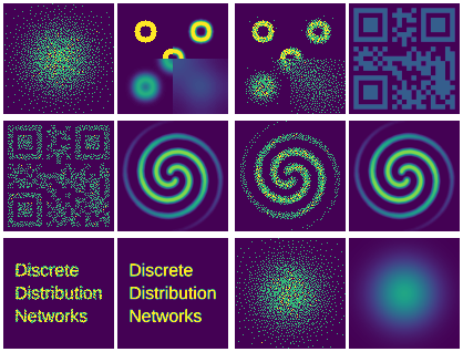
This GIF demonstrates the optimization process of DDN for 2D probability density estimation:
- Left image: All samples that can currently be generated
- Right image: Target probability density map
- For demonstration purposes, the target probability density maps switch periodically. Names and sequence of target probability maps:
blur_circles->QR_code->spiral->words->gaussian->blur_circles(same at beginning and end, completing a cycle)
- Therefore DDN continuously optimizes parameters to fit new distributions
- Optimizer: Gradient Descent with Split-and-Prune
- This only shows experimental results with 1,000 nodes; for a clearer and more comprehensive view of the optimization process, see the 2D Density Estimation with 10,000 Nodes DDN page
- The experiment code is in sddn/toy_exp.py, and the experimental environment is provided by the distribution_playground library, feel free to play with it yourself
Contributions of this paper:
- We introduce a novel generative model, termed Discrete Distribution Networks (DDN), which demonstrates a more straightforward and streamlined principle and form.
- For training the DDN, we propose the Split-and-Prune optimization algorithm, and a range of practical techniques.
- We conduct preliminary experiments and analysis on the DDN, showcasing its intriguing properties and capabilities, such as zero-shot conditional generation without gradient and distinctive 1D discrete representations.
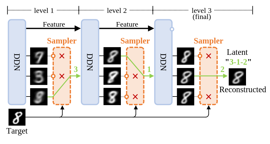
Left: Illustrates the process of image reconstruction and latent acquisition in DDN. Each layer of DDN outputs
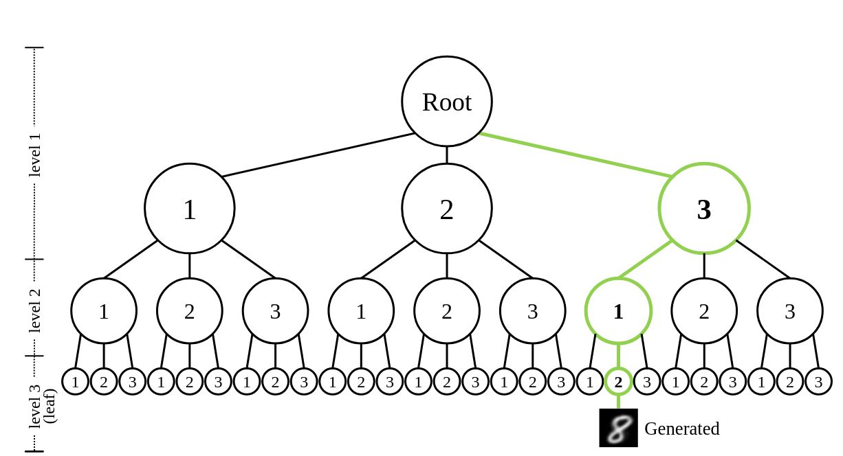
Right: Shows the tree-structured representation space of DDN's latent variables. Each sample can be mapped to a leaf node on this tree.
Reviews from ICLR:
I find the method novel and elegant. The novelty is very strong, and this should not be overlooked. This is a whole new method, very different from any of the existing generative models.
This is a very good paper that can open a door to new directions in generative modeling.
We introduce a novel generative model, the Discrete Distribution Networks (DDN), that approximates data distribution using hierarchical discrete distributions. We posit that since the features within a network inherently capture distributional information, enabling the network to generate multiple samples simultaneously, rather than a single output, may offer an effective way to represent distributions. Therefore, DDN fits the target distribution, including continuous ones, by generating multiple discrete sample points. To capture finer details of the target data, DDN selects the output that is closest to the Ground Truth (GT) from the coarse results generated in the first layer. This selected output is then fed back into the network as a condition for the second layer, thereby generating new outputs more similar to the GT. As the number of DDN layers increases, the representational space of the outputs expands exponentially, and the generated samples become increasingly similar to the GT. This hierarchical output pattern of discrete distributions endows DDN with unique properties: more general zero-shot conditional generation and 1D latent representation. We demonstrate the efficacy of DDN and its intriguing properties through experiments on CIFAR-10 and FFHQ.
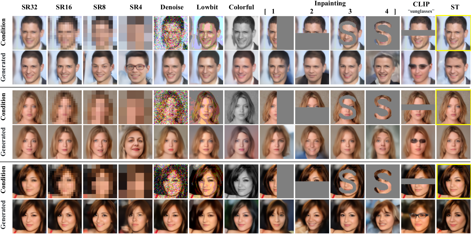
DDN enables more general zero-shot conditional generation. DDN supports zero-shot conditional generation across non-pixel domains, and notably, without relying on gradient, such as text-to-image generation using a black-box CLIP model. Images enclosed in yellow borders serve as the ground truth. The abbreviations in the table header correspond to their respective tasks as follows: “SR” stands for Super-Resolution, with the following digit indicating the resolution of the condition. “ST” denotes Style Transfer, which computes Perceptual Losses with the condition.
Overview of Discrete Distribution Networks
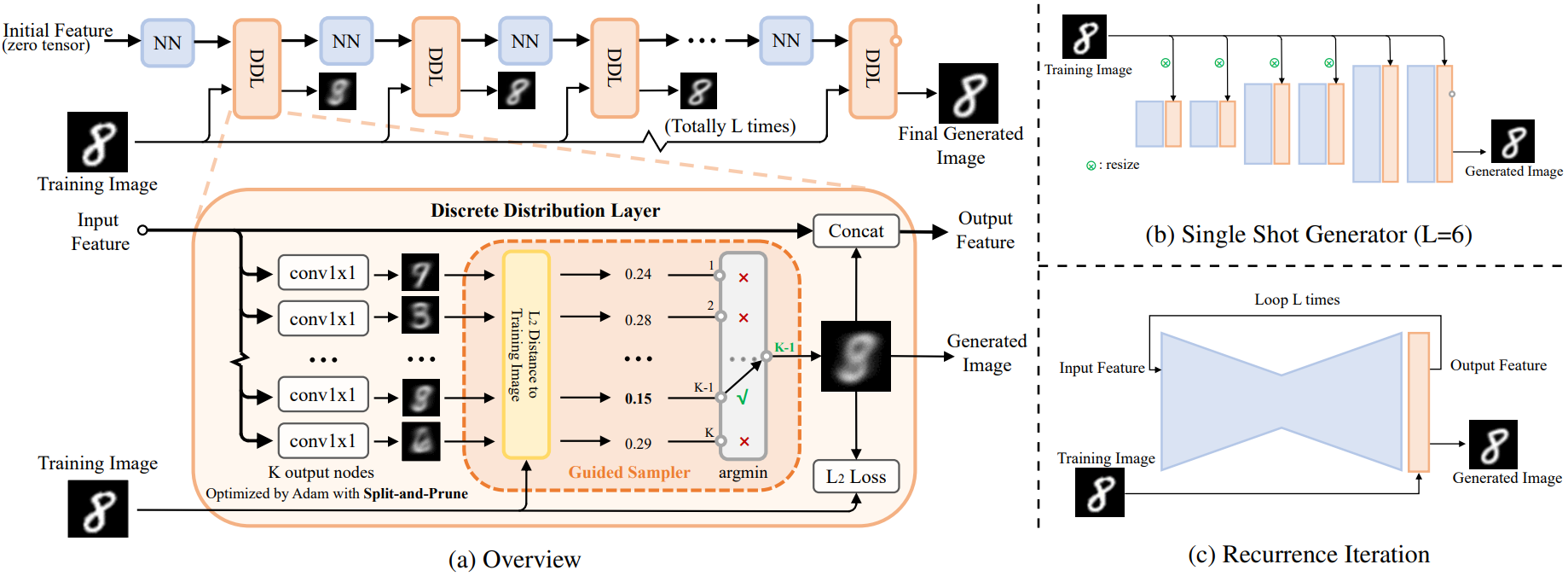
(a) The data flow during the training phase of DDN is shown at the top. As the network depth increases, the generated images become increasingly similar to the training images. Within each Discrete Distribution Layer (DDL),
The DDN model consists of
Here,
Toy examples for two-dimensional data generation
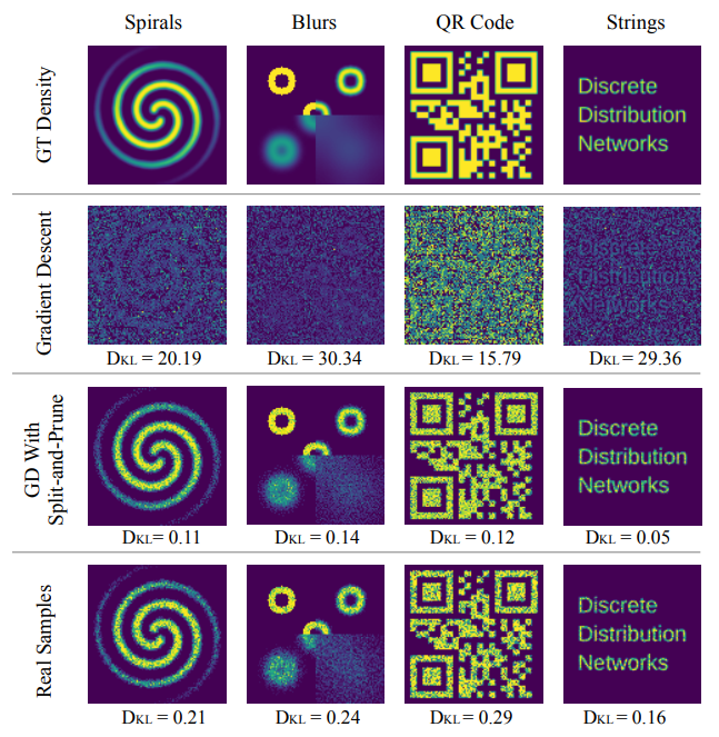
The numerical values at the bottom of each figure represent the Kullback-Leibler (KL) divergence. Due to phenomena such as “dead nodes” and “density shift”, the application of Gradient Descent alone fails to properly fit the Ground Truth (GT) density. However, by employing the Split-and-Prune strategy, the KL divergence is reduced to even lower than that of the Real Samples. For a clearer and more comprehensive view of the optimization process, see the 2D Density Estimation with 10,000 Nodes DDN page.
Zero-Shot Conditional Generation guided by CLIP
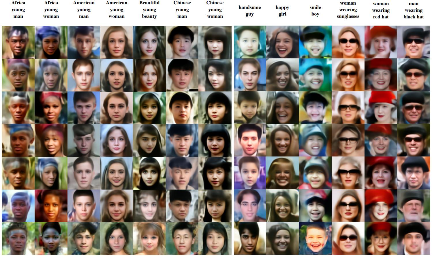
The text at the top is the guide text for that column.
Conditional DDN performing coloring and edge-to-RGB tasks
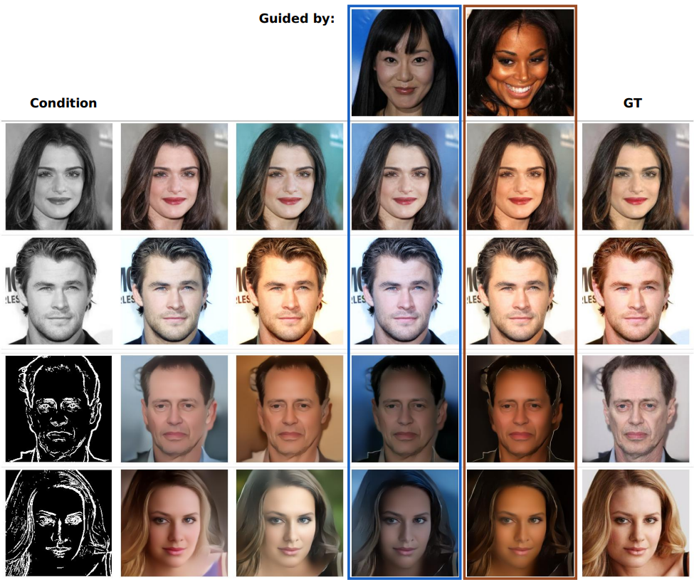
Columns 4 and 5 display the generated results under the guidance of other images, where the produced image strives to adhere to the style of the guided image as closely as possible while ensuring compliance with the condition. The resolution of the generated images is 256x256.

Online DDN coloring demo
To demonstrate the features of DDN conditional generation and Zero-Shot Conditional Generation.
Hierarchical Generation Visualization of DDN
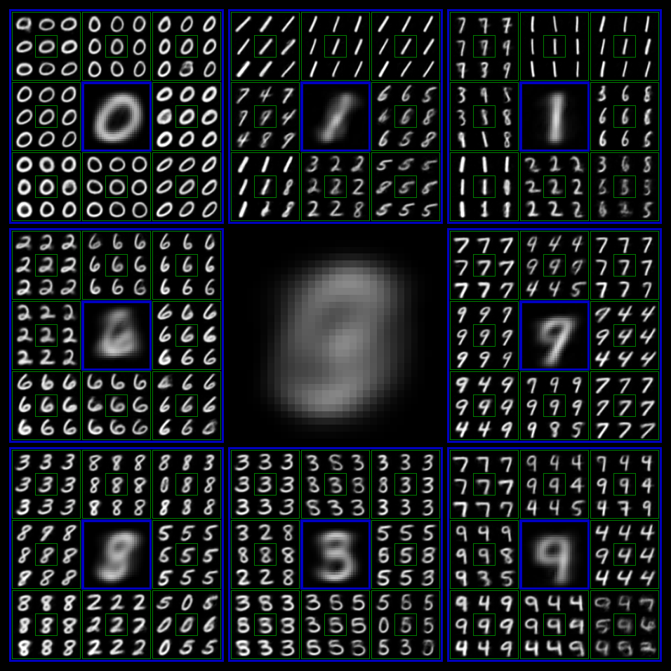
We trained a DDN with output level
Uncompressed raw backup of this video is here: DDN_latent_video
The following content contains personal opinions and is not included in the original paper
Future Research Directions
Based on the current state of DDN, we speculate on several possible future research directions. These include improvements to DDN itself and tasks suitable for the current version of DDN. Due to my limited perspective, some of these speculations might not be accurate:
Improving DDN through hyperparameter tuning, exploratory experiments, and theoretical analysis:
The total time spent developing DDN was less than three months, mostly by a single person. Therefore, experiments were preliminary, and there was limited time for detailed analysis and tuning. There is significant room for improvement.Scaling up to ImageNet-level complexity:
Building a practical generative model with Zero-Shot Conditional Generation as a key feature.Applying DDN to domains with relatively small generation spaces.
- Conditional training tasks where the condition provides rich information, such as image colorization and super-resolution.
- Generative models for discriminative tasks, such as depth estimation, optical flow estimation, and pose estimation.
- Robotics applications, where DDN could replace diffusion models in Diffusion Policy and Decision Diffuser frameworks.
- In these domains, DDN has advantages over diffusion models:
- Single forward pass to obtain results, no iterative denoising required.
- If multiple samples are needed (e.g., for uncertainty estimation), DDN can directly produce multiple outputs in one forward pass.
- Easy to impose constraints during generation due to DDN's Zero-Shot Conditional Generation capability.
- DDN is fully end-to-end differentiable, enabling more efficient optimization when integrated with discriminative models or reinforcement learning.
Applying DDN to non-generative tasks:
- DDN naturally supports unsupervised clustering. And its unique latent representation could be useful in data compression, similarity retrieval, and other areas.
Using DDN's design ideas to improve existing generative models:
- For example, the first paper citing DDN, DDCM, applied DDN's idea of constructing a 1D discrete latent to diffusion models.
Applying DDN to language modeling tasks:
- We made an initial attempt to combine DDN with GPT, aiming to remove tokenizers and let LLMs directly model binary strings. In each forward pass, the model adaptively adjusts the byte length of generated content based on generation difficulty (naturally supporting speculative sampling).
Common Questions About DDN
Q1: Will DDN require a lot of GPU memory?
DDN's GPU memory requirements are slightly higher than conventional GAN generator using the same backbone architecture, but the difference is negligible.
During training, generating
samples is only to identify the one closest to the ground truth, and the unselected samples do not retain gradients, so they are immediately discarded after sampling at the current layer, freeing up memory. In the generation phase, we randomly sample an index from
and only generate the sample at the chosen index, avoiding the need to generate the other samples, thus not occupying additional memory or computation.
Q2: Will there be a mode collapse issue?
No. DDN selects the output most similar to the current GT and then uses the
loss to make it even more similar to the GT. This operation naturally has a diverse tendency, which can "expand" the entire generation space. Additionally, DDN supports reconstruction. Figure 14 in the original paper shows that DDN has good reconstruction performance on the test set, meaning that DDN can fully cover the target distribution.
The real issue with DDN is not mode collapse but attempting to cover a high-dimensional target distribution that exceeds its own complexity, leading to the generation of blurry samples.


